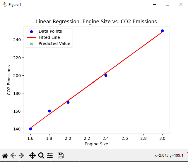
As we have learned in our previous chapter about regression, if you did not go through it, please do it is recommended. So in this chapter, we will discuss one type of regression, which is Simple Linear Regression; another is Multiple Linear Regression, which we will discuss in the next chapter; ok, don’t worry about that.

What is Simple Linear Regression

Now let’s discuss Simple linear regression. It is a fundamental technique in predictive modeling in which our model should predict a value. It allows us to predict a continuous target variable that has a continuous value based on a single independent variable. In this chapter, we’ll use an example dataset related to the CO2 emissions of various cars to understand the basic concept of Simple Linear Regression. In more, Simple linear regression involves two key variables: the dependent variable (target) and the independent variable(our feature). The goal is to establish a linear relationship between these variables(i.e how our dependent variable are dependent on our independent variable).

Purpose of Simple Linear Regression

Linear regression aims to find the best-fitting line that represents the relationship between the variables(dependent and independent variable). For instance, if we’re predicting CO2 emission(dependent variable) of a car based on engine size(independent variable), the line should capture this relationship.

Interpreting the Line

The line’s equation, y = mx + b, allows us to predict the target variable (y) based on the independent variable (x). In this equation, “m” is the slope of the line, and “b” is the y-intercept we also do implementation of it in python don’t worry.

How to Calculating Coefficients in Simple Linear Regression

To find the slope and intercept of the line, we calculate the coefficients theta_1 (slope) and theta_0 (intercept). These coefficients determine the line’s position and steepness.

How to Minimize Errors in Linear Regression

We may or may not find some errors we see in implementation of this algorithm in python but if we have some error, We evaluate the accuracy of the line by calculating residuals, which are the differences between actual and predicted values. The Mean Squared Error (MSE) quantifies how well the line fits the data. So what it would do, it reduce our error and the prediction which our model make is almost accurate i hope you got it.

Optimizing the Line in Linear Regression

As our objective is to minimize or you can say reduce the MSE(Mean Squared Error) by adjusting theta_0 and theta_1. We can achieve this through mathematical formulas or optimization techniques which should help us to reduce our error. Their are built-in libraries in Python which can do this for us such as Sk-Learn. will see in implementation don’t worry.

How to find co-efficient in Linear Regression mathematically

For simple linear regression, we can directly estimate theta_0 and theta_1 mathematically, using equations such as MSE(Mean Squared Error) based on the mean of the independent and dependent variables. These equations yield the intercept and slope.

How to use Coefficients for Prediction in Linear Regression

With calculated coefficients, we construct the linear regression equation. This equation allows us to predict the target variable for new data points.

How to do Linear Regression in Python

Here’s a step-by-step implementation of simple linear regression in Python using the numpy library for calculations and sklearn for linear regression & matplotlib for visualization of data.

import numpy as np
import matplotlib.pyplot as plt
from sklearn.linear_model import LinearRegression

# Sample data: engine size and corresponding CO2 emissions
engine_size = [1.8, 2.4, 2.0, 3.0, 1.6]
co2_emissions = [160, 200, 170, 250, 140]

# Reshape data for modeling
X = np.array(engine_size).reshape(-1, 1)  # Independent variable (engine size)
y = np.array(co2_emissions)  # Dependent variable (CO2 emissions)

# Create a linear regression model
model = LinearRegression()
model.fit(X, y)

# Predict CO2 emissions for a new car with engine size 2.4
new_engine_size = np.array([2.4]).reshape(-1, 1)
predicted_emission = model.predict(new_engine_size)

# Visualize the data points and the fitted line
plt.scatter(X, y, color='blue', label='Data Points')
plt.plot(X, model.predict(X), color='red', label='Fitted Line')
plt.scatter(new_engine_size, predicted_emission, color='green', marker='x', label='Predicted Value')

plt.xlabel('Engine Size')
plt.ylabel('CO2 Emissions')
plt.title('Linear Regression: Engine Size vs. CO2 Emissions')
plt.legend()
plt.show()

print(f"Predicted CO2 Emissions: {predicted_emission}")

Output

Predicted CO2 Emissions: [202.46753247]

Conclusion

In last by concluding all above i want to say that, Simple linear regression is a powerful tool or you can say algorithm for predicting continuous values based on one independent variable. It forms the foundation of more advanced machine learning techniques and is a valuable addition to any data scientist’s toolkit.

Link: https://Codelikechamp.com

Medium Link: Follow me on Medium

Linkedin Link: Follow me on Linkedin